FMRI
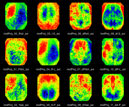
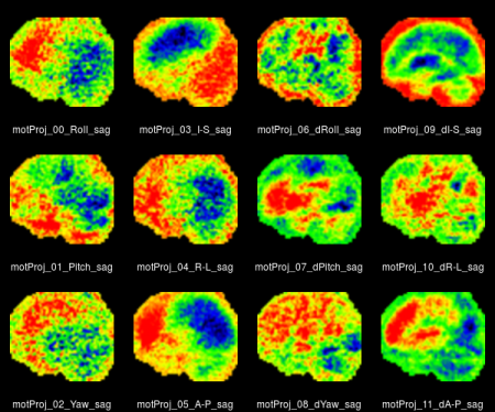
Participant in-scanner motion is one of the prominent sources of artefacts in fMRI data. This was recognized as an issue in fMRI long ago (Hajnal et al., 1994; Friston et al., 1996). Due to the spin excitation history issue already pointed out by Bullmore et al., 1999(PDF), motion has complex effects on the signal - including increases, decreases or complex waveforms, depending on factors such as the timing, duration and trajectory of motion (Power et al., 2015, Byrge and Kennedy 2018). Crucially, motion can substantially affect estimates of functional connectivity (Power et al., 2012; Satterthwaite et al., 2012). Initial motion-correction approaches involved regression of motion parameters and their derivatives from voxel-wise BOLD time series (Friston et al., 1996), or regression of the average or "global" signal (Aguirre et al., 1998; for a recent review, see Murphy and Fox, 2017). Later solutions included censoring of motion-affected frames (Power et al., 2012), removal of non-BOLD (artefactual) signal using independent component analysis applied to multi-echo fMRI data, based on the dependence of the BOLD signal on echo time (Kundu et al., 2012, 2013), or "despiking" of motion-related non-stationary events from a wavelet decomposition of the signal (Patel et al., 2014). The latter method was subsequently extended to provide revised estimates of voxel-wise effective degrees of freedom (df) of the BOLD time series, which due to denoising are lower than the nominal N(df ) = N(time-points), and which affect estimates of edge probability when incorporated into network analysis (Patel and Bullmore, 2016).
Other prominent artifacts, particularly in fMRI, relate to respiration, vasculature and arousal (e.g.: Murphy et al., 2013; Caballero-Gaudes and Reynolds, 2017).
Quality control
Multiple diagnostic measures can be investigated during quality control of fMRI data, to ensure that the processed data are maximally free of motion-related (or other) artefacts. The following steps apply across types of fMRI acquisition (e.g.: single- or multi-echo data) and across processing pipelines.
Framewise Displacement
One key quantity used for diagnostic purposed is the framewise displacement (FD), a subject-specific time-series indexing an overall estimate of movement over time. During processing, re-alignment of scans is used to estimate 6 motion parameters for each participant (3 translation parameters and 3 rotation parameters). Subsequently, these were used to calculate an overall estimate of motion - the framewise displacement (FD), defined as the sum of the absolute temporal derivatives of the six motion parameters, following conversion of rotational parameters to distances by computing the arc length displacement on the surface of a sphere with radius 50 mm (as in Power et al. (2012) and Patel et al. (2014)):
where d denotes translation distances {x,y,z}, and r denotes rotation angles {α,β,γ}. For each participant, a single (scalar) estimate of overall motion, the mean FD, can be calculated by averaging the FD time series.
The values of FD should be inspected - both the mean FD, as well as subject-specific distributions of FD over time. The exclusion of a small subset of high-motion participants can substantially improve overall data quality, and decrease the strength of the relationship between motion and functional connectivity across subjects, which can be driven by a few high-motion outliers. There is no universally accepted threshold for movement, but past studies have excluded participants both on the grounds of high average FD, and of a high proportion of motion-contaminated time points. For example, Gu et al. (2015) excluded participants with mean FD > 0.2 mm, and those with > 20/124 volumes with FD > 0.25 mm. The thresholds to choose are likely to be study-specific - but should be based on the knowledge that even seemingly very small magnitude of motion (< 0.05 mm) can have artefactual impacts on the data (Byrge and Kennedy, 2018).
Relationship of Framewise Displacement to Functional Connectivity
The mean FD can be used to detect potential residual relationships between functional connectivity (FC, usually defined as the cross-correlation between processed fMRI time-series between pairs of regions) and movement, across subjects. This can be evaluated at three levels: - globally (averaging FC over the upper triangular part of the correlation matrix) - regionally (averaging FC for each node, by calculating the average over rows (or columns) of the correlation matrix) - edge-wise (at each entry of the correlation matrix) Additionally, the relationship of the matrix of edge-wise correlations between FC and motion (across participants) to the matrix of Euclidean distances between pairs of regional centroids can be studied. In the BMU, this is known as the "Satterthwaite plot", based on the introduction of this diagnostic tool by Ted Satterthwaite (Fig. 1 in Satterhwaite et al. (2012)).
Ideally, the magnitude of FC should not correlate with FD, at any of the three levels. The ideal outcome of the Satterthwaite plot (with distance on the x-axis, and the across-participant correlation between edge-wise FC and mean FD on the y-axis) is a horizontal line - indicating that edges spanning different distances are not differentially affected by motion in the processed data, with a y-axis intercept of 0 - indicating that at the edge level, there is no relationship between participant motion and FC.
If residual relationships remain after data processing, these can potentially be regressed out across participants, by regressing FC at each edge against mean participant FD and retaining the residuals as the new FD-corrected FC (ideally, intercepts of this regression should be added back to the residuals, to retain the average variability in FC across edges, and to simplify interpretation of the corrected quantities). This additional step has been applied for example in Gu et al. (2015).
Lagged effects of motion on fMRI time-series
An additional quality control plot has been proposed by Byrge and Kennedy (2018). The authors investigated whether movements of similar magnitude produce structured artefactual effects on the fMRI time-series. Creating a diagnostic plot of this effects involves binning all time-points (in each participant) according to the magnitude of motion at that time-point, based on the FD time-series. The bins do not have to be of equal size, but should not overlap - for example, Byrge and Kennedy apply the following: bin 1 = motion of 0.00-0.05 mm, bin 2 = motion of 0.05-0.10 mm, ..., bin N = motion of 0.90-1.5 mm. Subsequently, equally long segments of (processed) fMRI time-series (eg: 25 TRs) following each instance of motion are averaged within each bin. This analysis can be conducted using the global signal (across subjects), or regional signal (within subjects). The ideal outcome, when applied to processed fMRI data, should be flat time-series (of average BOLD signal following motion events of similar magnitudes) within each bin of motion magnitude, indicating a lack of structured effects of motion on the BOLD signal.
In practice, following standard processing steps, movement does produce structured effects on the BOLD signal, which extend far in time beyond the displacement (~ up to 40 seconds) and are non-linear (small movements produce an initial undershoot followed by an overshoot, which is progressively reversed as the magnitude of motion increases). In practice, this means that these effects cannot be adequately controlled by removal of motion-related frames (a.k.a. "scrubbing"), or regression of the motion time-series from the BOLD signal (which only leads to correction of zero-lag effects).
For details on these diagnostic plots, and a Matlab implementation, see Byrge and Kennedy (2018).
ME-ICA processing for NSPN and BIODEP
The following pipeline describes processing steps for multi-echo ICA (ME-ICA) data, as agreed by Manfred, Frantisek and others in May 2018. This is the pipeline applied to NSPN and BioDep projects.
Briefly, the processing pipeline includes the following steps:
- copy the structural brain image and the multi-echo EPI timeseries into the individual subject folder
- run the MEICA script specifying the structural image with the -a argument and the functional images with the -d argument. Additionally you will need to know the actual echo times for the respective functional images and specify them with the -e argument.
- importantly, the --smooth argument should not be used because it interferes with the MEICA artefact detection heuristics by mixing components
The current version of the ME-ICA script to be run is located on the BCNI server at: "/home/rr480/Code/MATLAB/fMRI/MEICA/meica_manfred_2018_05_10/meica.py". This includes the options listed below (some of which are specific to NSPN data). For a detailed description of all processing steps, see MEICA.
 -d 'echo[1,2,3].nii'
 -a 'brainmask.nii'
 -e 13.0,30.55,48.1
 --TR=2.43
 --tpattern=seq-z
 -b 15s
 --fres=2.5
 --mask_mode='anat'
 --no_skullstrip
 --OVERWRITE
- the output from MEICA is very rich and will give you a large number of files that can be used as a diagnostic for quality control. See Matilde's excellent QC summary on the subject.
- the main output however is the one file with suffix "_medn.nii.gz" which stands for "Multi Echo DeNoised"
- even though MEICA can remove many of the artefacts in the functional data by identifying non-BOLD components, it's not perfect and it can be shown that some motion artefacts remain even in the denoised output (cf. "Satterthwaite" and "Byrge" plots above).
- it could therefore be beneficial to regress out motion parameters (or a summary, such as FD; but either will only remove the zero-lag component) or a nuisance timeseries extracted from the CSF and WM regions of the brain which are not expected to display any BOLD signal related to legitimate neuronal activity.
See Behzadi et al 2007 and Caballero-Gaudes and Reynolds, 2017 for a more detailed treatment of the subject. - at this point the cleaned data can be parcellated using your favourite template such as AAL, Desikan, Glasser et al. to extract a set of ROI timeseries to be used for subsequent connectivity and graph analysis.
The arguments above will keep all MEICA output in "native" space rather than transform it into a standardized space such as MNI because an individual surface based Freesurfer template will be used in NSPN.
The generic MEICA page shows how to get output in standard space if needed. - the ROI timeseries are wavelet filtered to wavelet scales 2-3 in order to minimise/mitigate correlations between low frequency events in the time series and slow drifts of the head during scanning. (For NSPN data, this is performed using the MODWT with Daubechies 4 wavelet and reflection boundary condition. Wavelet coefficients for all unwanted scales (i.e.: scales other than 2 and 3) are set to 0, as are the the scaling coefficients, before the wavelet filtered time-series is reconstituted using the inverse MODWT. The correlation matrix is then generated in the time-domain, using the filtered time-series.)
- the matrix of correlations between all ROI pairs is used as a connectivity metric
- please refer to the section on Network Construction on the main page for the next steps.


